Computational Optics

Conventional imaging systems employ compound refractive lens systems that are typically hand-engineered for image quality in isolation of the downstream camera task. Departing from this design paradigm, a growing body of work in computational photography [Haim et al. 2018; Horstmeyer et al. 2017] has explored the design of specialized lens systems with diffractive optical elements (DOEs).

As a specific example, we consider end-to-end computational optics that jointly optimize a diffractive optical element (DOE) and an image reconstruction algorithm, where the observation \(y\) is obtained by convolving a clear image \(x\) by the point spread function (PSF) of DOE as,

\[y = D\left(x;\, \theta_{DOE} \right) + \epsilon,\]

where \(D(\cdot; \theta_{DOE})\) indicates a shift-invariant convolution process with an optical kernel, i.e., PSF, derived from a DOE image formation model parameterized by \(\theta_{DOE}\), and \(\epsilon\) is measurement noise, e.g., Poissionian-Gaussian noise. To reconstruct the target image \(x\) from noise-contaminated measurements \(y\), we minimize the sum of a data-fidelity \(f\) and regularizer term \(r\) as

\[\mathop{\mathrm{min}}_{x \in \mathbb{R}^n} ~ f \left( D\left(x;\, \theta_{DOE} \right) \right) + r \left(x ; \, \theta_r \right).\]

In this tutorial, we will show three different approaches to solving this problem, including

1. Green-focused Fresnel lens deconvolution with a plug-and-play proximal algorithm in \(\nabla\)-Prox.

2. Conventional joint optimization of the DOE model and black-box deep deconvolution neural network. [Metzler et al. 2020]

3. Joint optimization of the DOE model and differentiable proximal solver in \(\nabla\)-Prox.

# uncomment the following line to install dprox if your are in online google colab notebook
# !pip install dprox

import os
import torch
import torch.nn as nn
from dprox import *
from dprox.utils import *
from dprox.contrib.optic import *

DOE with baseline profile (green-focused Fresnel lens)

Let us first build a DOE model. Note that you can adjust the physical optical setup parameters using the DOEModelConfig class. Please assure that you have some domain knowledge of Fourier Optics

config = DOEModelConfig()
rgb_collim_model = build_doe_model(config=config)

By cropping the center region of the point spread function (PSF) of the baseline DOE model, we can visualize it as shown below.

fresnel_phase_c = build_baseline_profile(rgb_collim_model)
psf = rgb_collim_model.get_psf(fresnel_phase_c)
psf_baseline = crop_center_region(normalize_psf(to_ndarray(psf, debatch=True), clip_percentile=0.01, bandwise=False), size=150)
imshow(psf_baseline, titles=["PSF of a green-focused Fresnel lens"], off_axis=True)

Next, let us load a sample image and generate the blurred observation with the baseline DOE model.

gt = load_sample_img(hf.load_path('examples/optics/sample.png'))

sigma = 7.65 / 255
noise = torch.randn(*gt.shape, device=gt.device) * sigma
psf = rgb_collim_model.get_psf(fresnel_phase_c)
inp_baseline = img_psf_conv(gt, psf, circular=True) + noise
imshow(gt, inp_baseline, titles=['Original scene', 'Image through a green-focused Fresnel lens'], off_axis=True)

We can use the plug-and-play proximal algorithm to reconstruct the clean image from the blurred observation.

Here, we show an example of how to solve it with ADMM and a deep image prior in \(\nabla\)-Prox.

x = Variable()
y = Placeholder()
PSF = Placeholder()
data_term = sum_squares(conv_doe(x, PSF, circular=True), y)
reg_term = deep_prior(x, denoiser='ffdnet_color')
solver = compile(data_term + reg_term, method='admm')  # compile the optimization problem into an ADMM solver

inp = inp_baseline.float()
y.value, PSF.value = inp, psf
max_iter = 10
rhos, sigmas = log_descent(49, 7.65, max_iter, sigma=max(0.255 / 255, sigma))  # set inner loop parameters using a log descent policy
out_baseline = solver.solve(x0=inp, rhos=rhos, lams={reg_term: sigmas}, max_iter=max_iter)

imshow(out_baseline, out_baseline[:,:,460:660,140:340], titles=[f'recovery (PSNR: {psnr(out_baseline, gt):.3f})', 'zoom in'], off_axis=True)

The results show that the naive DOE model (green-focused Fresnel lens) does not work well with existing post-processing techniques, such as the proximal algorithm we used here. To further increase the interaction between the imaging model and processing algorithms, we can jointly optimize them.

Conventional Joint Optimization of DOE Model and Deep Deconvolution Network

In DeepOptics-UNet, Metzler et al. propose jointly optimizing the DOE model and a post-deconvolution network. This results in a learned DOE model whose PSF can be visualized as follows. The learned PSF is quite different from the previous one, which focuses more on colors instead of solely a green channel.

from dprox.contrib.optic import U_Net
device = torch.device('cuda:0')
solver = U_Net(3,3).to(device)
rgb_collim_model = build_doe_model().to(device)

ckpt = hf.load_checkpoint('computational-optics/joint_deepoptics_unet.pth')
rgb_collim_model.load_state_dict(ckpt['model'])
solver.load_state_dict(ckpt['solver'])

psf = rgb_collim_model.get_psf()
psf_unet = crop_center_region(normalize_psf(to_ndarray(psf, debatch=True), clip_percentile=0.01))
imshow(psf_unet, titles=["DOE's PSF jointly optimized with a UNet"], off_axis=True)

To see the performance of joint optimization, we can capture/generate an observation and compare it to the reconstruction result of the deconvolution network.

gt = gt.to(device).float()
psf = rgb_collim_model.get_psf()
inp = img_psf_conv(gt, psf, circular=True)
inp_unet = inp + torch.randn(*inp.shape, device=inp.device) * sigma
out_unet = solver(inp_unet)
imshow(inp_unet, out_unet, out_unet[:,:,460:660,140:340], titles=['measurement', f'output (PSNR: {psnr(out_unet, gt):.3f})', 'zoom in'], off_axis=True)

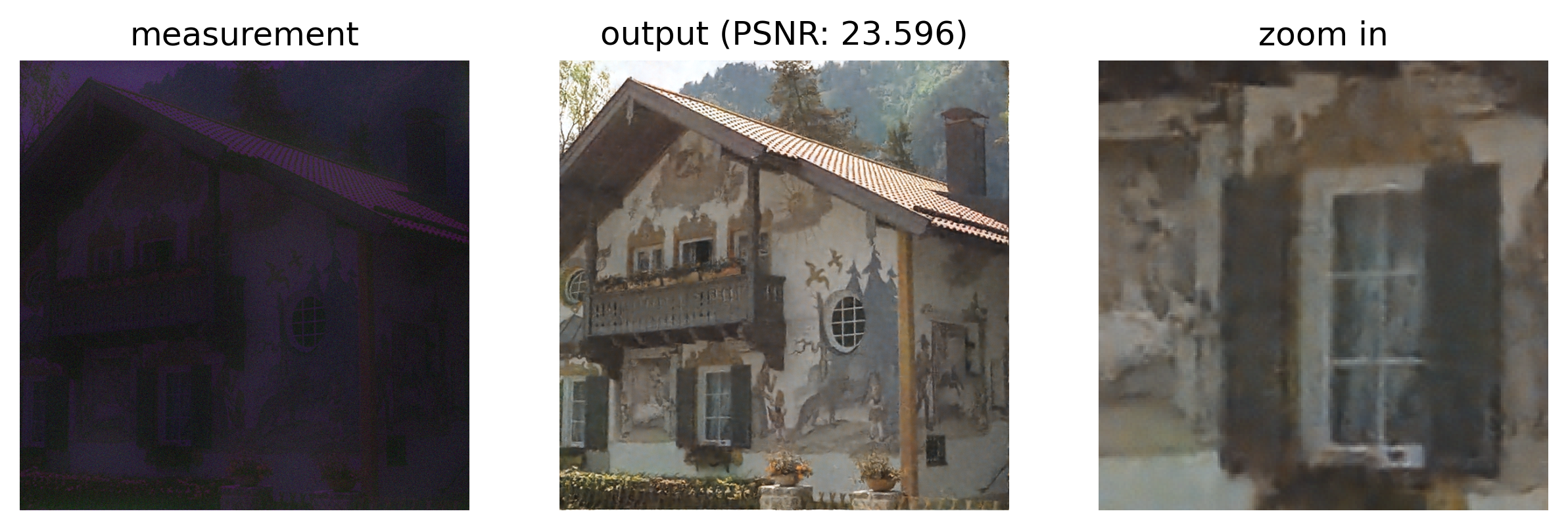
👻 Oops! The results are much better, which demonstrates the benefit of joint optimization.

The approach above jointly optimizes the DOE model and a black-box deconvolution network. Now, let us jointly optimize the DOE model with a formal optimization deconvolution algorithm, e.g., a proximal algorithm.

DOE with Learned Profile in \(\nabla\)-Prox

\(\nabla\)-Prox builds differentiable proximal solvers that can be used to jointly optimize every input to the solver, e.g., the DOE model.

For simplicity, we provide the learned DOE model by \(\nabla\)-Prox. Its training code can be found in computational_optics.

# load learned doe model
rgb_collim_model.rhos = nn.parameter.Parameter(torch.zeros((max_iter)))
rgb_collim_model.sigmas = nn.parameter.Parameter(torch.zeros((max_iter)))
rgb_collim_model.load_state_dict(hf.load_checkpoint('computational_optics/joint_dprox.pth')['model'])

# visualize point spread function
psf = rgb_collim_model.get_psf()
psf_dprox = crop_center_region(normalize_psf(to_ndarray(psf, debatch=True), clip_percentile=0.01))
imshow(psf_dprox, titles=["DOE's PSF jointly optimized with a proximal solver"], off_axis=True)

Interestingly, the above visualization highlights that the optimized PSF resulting from the end-to-end optimization problem drastically differs from the one optimized with a UNet post-processor.

The phase pattern we learn focuses the three wavelength bands as highly chromatic PSFs for each channel, that is, the red, green, and blue PSFs only focus on the specific channel while spreading out energy for other wavelengths over the entire sensor.

By spatially separating the corresponding phase patterns, our co-designed network can find these chromatic PSFs. As such, \(\nabla\)-Prox allows us to find a novel point in the design space – turning an out-of-focus deconvolution problem into a transverse chromatic alignment problem. 🙀

# generate input
gt = gt.to(device).float()
psf = rgb_collim_model.get_psf()
inp = img_psf_conv(gt, psf, circular=True)
inp_dprox = inp + torch.randn(*inp.shape, device=inp.device) * sigma

# build solver
x = Variable()
y = Placeholder()
PSF = Placeholder()
data_term = sum_squares(conv_doe(x, PSF, circular=True), y)
reg_term = deep_prior(x, denoiser='ffdnet_color')
solver = compile(data_term + reg_term, method='admm')

# solve the problem
y.value = inp_dprox
PSF.value = psf
with torch.no_grad():
    out_dprox = solver.solve(x0=inp_dprox,
                        rhos=rgb_collim_model.rhos,
                        lams={reg_term: rgb_collim_model.sigmas.sqrt()},
                        max_iter=max_iter)

imshow(inp, out_dprox, out_dprox[:,:,460:460+200,140:140+200], titles=['measurement', f'output (PSNR: {psnr(out_dprox, gt):.3f})', 'zoom in'], off_axis=True)

In a nutshell, the model-based proximal optimization solver compiled with \(\nabla\)-Prox finds a better local minimum with a significantly improved end-to-end loss, which validates the effectiveness of the differentiable pipelines we compile.

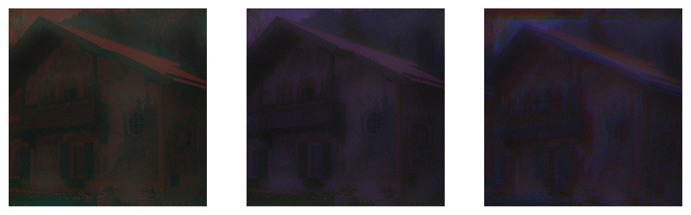
Wrap up the results

imshow(psf_baseline, psf_unet, psf_dprox, off_axis=True, titles=['Fresnel lens', 'DeepOptics-UNet', 'Ours'])
imshow(inp_baseline, inp_unet, inp_dprox, off_axis=True)
imshow(out_baseline, out_unet, out_dprox, off_axis=True)
imshow(out_baseline[:,:,460:460+200,140:140+200], out_unet[:,:,460:460+200,140:140+200], out_dprox[:,:,460:460+200,140:140+200], off_axis=True)
print('PSNR - Baseline: {} DeepOptics-Unet: {} Ours: {}'.format(psnr(gt, out_baseline), psnr(gt, out_unet), psnr(gt, out_dprox)))

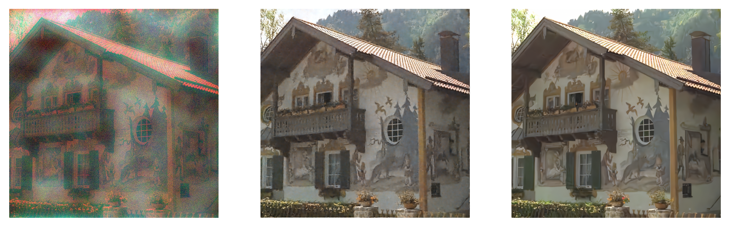
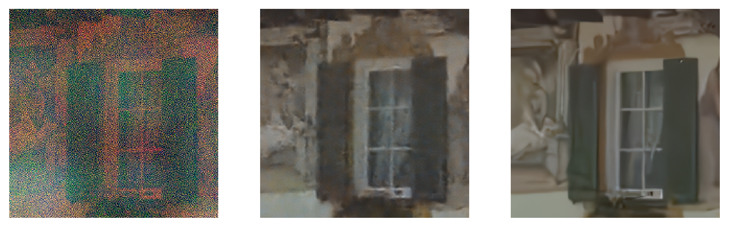
PSNR - Baseline: 15.985067266587896 DeepOptics-Unet: 23.59640974017188 Ours: 30.081977082831056

Reference

[Haim et al. 2018] Harel Haim, Shay Elmalem, Raja Giryes, Alex Bronstein, and Emanuel Marom. 2018. Depth Estimation From a Single Image Using Deep Learned Phase Coded Mask. IEEE Transactions on Computational Imaging 4 (2018), 298–310.

[Horstmeyer et al. 2017] Roarke Horstmeyer, Richard Y. Chen, Barbara Kappes, and Benjamin Judkewitz. 2017. Convolutional neural networks that teach microscopes how to image. ArXiv abs/1709.07223 (2017).

[Metzler et al. 2020] Christopher A Metzler, Hayato Ikoma, Yifan Peng, and Gordon Wetzstein. 2020. Deep optics for single-shot high-dynamic-range imaging. In Proceedings of the IEEE/CVF Conference on Computer Vision and Pattern Recognition. 1375–1385.