Learn the Basics of \(\nabla\)-Prox

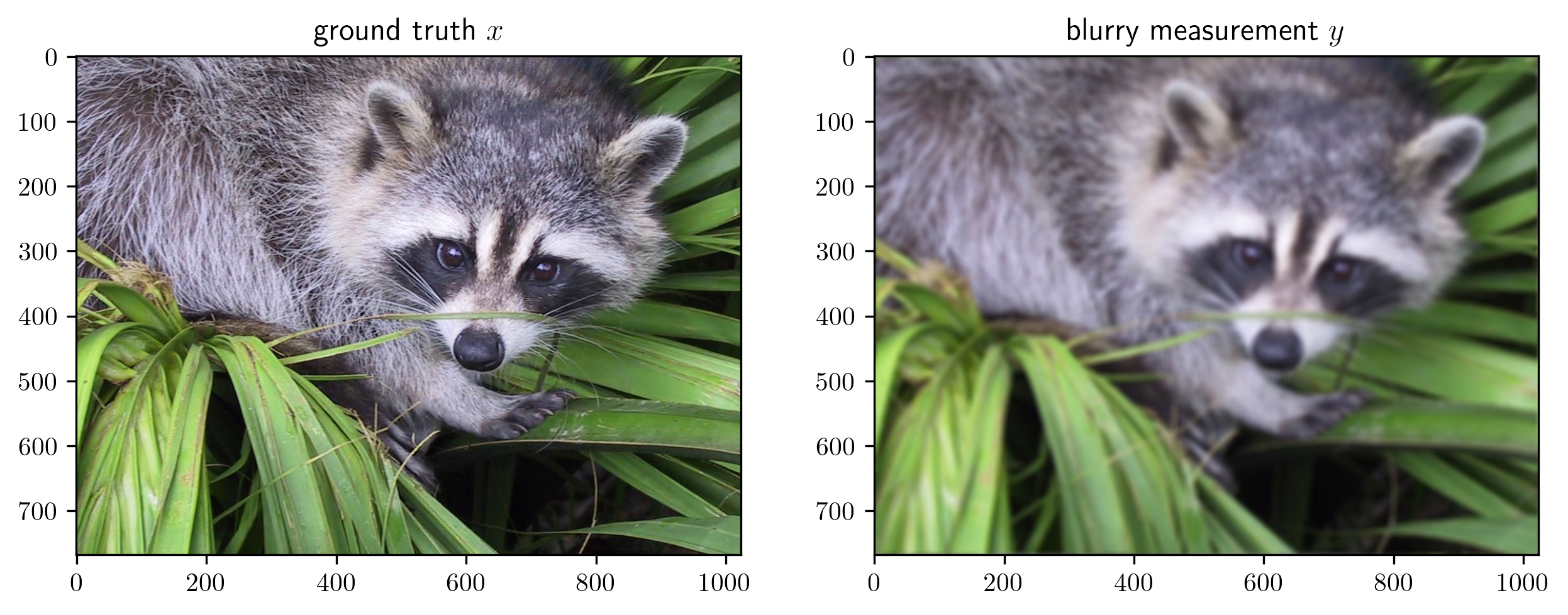
This tutorial introduces a complete proximal optimization workflow implemented in \(\nabla\)-Prox. For simplicity, we will use an image deconvolution problem as an example to demonstrate the functionalities of \(\nabla\)-Prox.

The goal of image deconvolution is to reconstruct the clear image \(x\) from the blurred observation \(y\) that is obtained by convolving \(x\) by the point spread function (PSF) as

\[y = D(x, \text{PSF})\]

where \(D\) denotes convolution operation.

To reconstruct the target image \(x\) from noise-contaminated measurements \(y\), we minimize the sum of a data-fidelity \(|| D(x) - y ||^2_2\) and regularizer term \(r\) as,

\[\mathop{\mathrm{min}}_{x \in \mathbb{R}^n} ~ || D(x) - y ||^2_2 + r (x ; \, \theta_r).\]

We consider a hybrid regularizer including (1) an implicit plug-and-play prior \(g(x; \theta_r)\) parameterized by \(\theta_r\) and (2) a non-negative constraint of the image.

\[r(x; \theta_r) = \lambda g(x; \theta_r) + I_{[0,\infty)},\]

Note: In order to run the following tutorial, please install the requirements following the Installation Tutorial

# uncomment the following line to install dprox if your are in online google colab notebook
# !pip install dprox

Import libraries

In the begining, we import all the necessary libraries.

from dprox import *
from dprox.utils import *
from dprox.contrib import *
import matplotlib.pyplot as plt
plt.rc('text', usetex=True)

Prepare Data

Then, let’s generate some sample data to play with.

img = sample('face')
psf = point_spread_function(ksize=15, sigma=5)
y = blurring(img, psf)
print(img.shape, y.shape)
imshow(img, y, titles=[r'ground truth $x$', r'blurry measurement $y$'])

torch.Size([1, 3, 768, 1024]) torch.Size([1, 3, 768, 1024])

Representing the Optimization Problem in \(\nabla\)-Prox

Given the blurry observation, our goal is to reconstruct the clear image by solving an optimization problem of the following form:

\[\mathop{\mathrm{min}}_{x \in \mathbb{R}^n} ~ || D(x) - y ||^2_2 + \lambda g(x; \theta_r) + I_{[0,\infty)}.\]

We can write this problem in \(\nabla\)-Prox with a very simple syntax following the math.

x = Variable()
data_term = sum_squares(conv(x, psf) - y)
prior_term = deep_prior(x, 'ffdnet_color')  # using a simple FFDNet denoiser as a deep plug-and-play prior
reg_term = nonneg(x)
objective = data_term + prior_term + reg_term
p = Problem(objective)

Basic Problem Solving

Solving the problem only requires calling the solve method with the desired algorithms, e.g., ADMM in this case.

One can also try other algorithms. The compatible methods and their reference performance are listed below:

Key	Method	Expected PSNR
admm	Alternative Direction Method of Multiplier	31.94
hqs	Half Qudratic Splitting	31.65
pc	Pock Chambolle	29.66
ladmm	Linearized ADMM	31.95

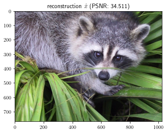
out = p.solve(method='admm', x0=y, pbar=True)
imshow(out, titles=[r'reconstruction $\hat{x}$ ' + f'(PSNR: {psnr(out, img):.3f})'])

100%|██████████| 24/24 [00:01<00:00, 16.13it/s]

In many cases, one needs to manually tune the hyperparameters of the algorithm to achieve better performance. For example, consider a slightly harder noisy deconvolution problem as

\[y = D(x, \text{PSF}) + \epsilon\]

where \(\epsilon\) denotes a small amount of Gaussian noise with intensity \(\sigma = \frac{5}{255}\).

y = blurring(img, psf) + np.random.randn(*img.shape).astype('float32') * 5/255.0
imshow(img, y, titles=[r'ground truth $x$', r'blurry and noisy measurement $y$'])

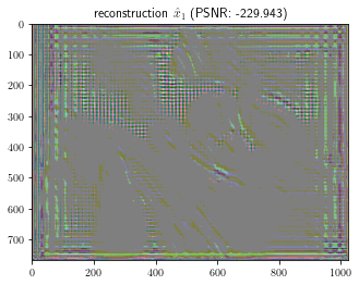
Again, let us solve the problem with \(\nabla\)-Prox. We can see that the default parameters diverge and fail to solve the problem.

x = Variable()
data_term = sum_squares(conv(x, psf) - y)
prior_term = deep_prior(x, 'ffdnet_color')
reg_term = nonneg(x)
objective = data_term + prior_term + reg_term
p = Problem(objective)
out = p.solve(method='admm', x0=y, pbar=True)
imshow(out, titles=[r'reconstruction $\hat{x}_1$ ' + f'(PSNR: {psnr(out, img):.3f})'])

100%|██████████| 24/24 [00:00<00:00, 26.08it/s]

To fix it, we have to manually tune the algorithm parameters. In \(\nabla\)-Prox, this can be achieved by passing extra keyword arguments to the solve method, e.g.,

out = p.solve(method='admm', x0=y, rhos=0.004, lams=0.02, max_iter=24, pbar=True)
imshow(out, titles=[r'reconstruction $\hat{x}_2$ ' + f'(PSNR: {psnr(out, img):.3f})'])

100%|██████████| 24/24 [00:00<00:00, 29.36it/s]

We should note that the manual parameter tuning is a tedious process. Different choices of parameters may significantly affect the performance. For example, by changing rhos to 0.1, the PSNR drops by 1.3 dB.

out = p.solve(method='admm', x0=y, rhos=0.1, lams=0.02, max_iter=24, pbar=True)
imshow(out, titles=[r'reconstruction $\hat{x}_3$ ' + f'(PSNR: {psnr(out, img):.3f})'])

100%|██████████| 24/24 [00:00<00:00, 29.43it/s]

In many cases, the optimal choice may vary for different inputs. Moreover, for real-world applications, we will not have the ground truth to evaluate the performance of different parameters for different inputs, which makes parameter tuning even harder.

To address it, \(\nabla\)-Prox incorporates the automatic parameter scheduler that can be learned via reinforcement learning. Please refer to the tutorial on automatic parameter scheduler for more details.